|
Image Acquisition and Reduction - by Ricky Leon Murphy:
Back to
Astrophotography
Image Acquisition
and Reduction:
Our software of choice
will be MaxImDL. This software is capable of controlling a CCD camera,
and performs some very powerful image edit using a wide variety of
tools. With this software, we are able to remove any bad or damaged
pixels, calibrate images using the bias and flat frames, create a color
composite, and perform photometry – which is the only method used to
create the data points on a CMD. In addition to MaxImDL, we will also
use Microsoft Excel to store the photometric data as well as perform
image calibration and create the actual diagram. The image reduction
process itself is a fairly simple concept, but time consuming. While the
attached appendix documents every step of the reduction process, a
guided tour is provided:
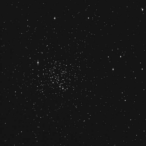
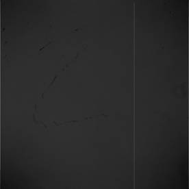
Each image
has, in addition to the actual image (or flat or bias), an area of
unexposed
 |
pixels used to store bias information. This area is called ‘overscan.’
Because we are calibrating various images using various filters,
the overscan area is of no use and must be removed. There is a
thin column of nothing on the far right of the image on the
left. This thin area is the overscan and is present in every
image provided by the McDonald Observatory. This area can be
mapped out within MaxImDL and applied to every image. In
addition to
the overscan, the
border of the entire image, which is one pixel in width, must
also be removed. This has been included in the map. |
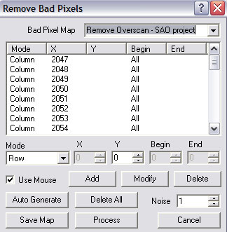 |
The remove bad
pixels tool under the process menu is able to
remember the selected pixels in one image. The unfortunate is
that every pixel has to be selected by the mouse, or entered by
hand – if you know the exact pixel location. In this case, I
renamed my map1 to Remove Overscan – SAO project. To apply this
map to other images, I open this tool and click the process
button.
|
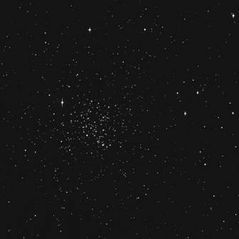 |
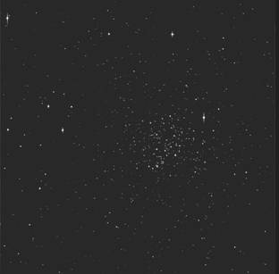
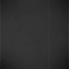
The result of the
overscan removal is seen here. Notice the dark area on the far
right is no longer present. This image of M67 is oriented
properly versus the mirrored image above. Once the overscan has
been removed from all cluster images, standard fields, bias and
flat images, the headers of each image must be fixed.
|
 |
 |
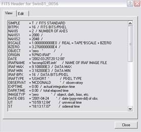
Looking at the view
menu within MaxImDL, there is a tool to view the fits header. Every
image captured on professional CCD cameras store important information
about the image captured. For example, the size of the chip, date of
image capture, duration of image capture, the airmass value, and filter
used is recorded in this header. Also, demographic, telescope type, and
astrometry information can also be a part of this header. Within this
header, the areas of overscan have been removed, and the image size has
been updated to reflect the actual image size (details are available in
the image reduction appendix). In the image above, the value ‘airmass’
is highlighted. This value is an important one as it is used to
determine the airmass value of the atmosphere. Every night, the quality
of the atmosphere (called the “seeing”) is given a numerical value. This
value also changes as the area photographed is closer to the horizon.
The airmass values included in the fits header will probably be
incorrect. The good news is there are airmass calculators available so
the correct airmass value can be found. The bias and flat field images
do not require a correct airmass value as no object is being
photographed through the atmosphere.
Once the overscan has
been removed and the fits headers correct, image calibration can begin.
As above, there is a detailed report of image reduction in the image
reduction diary; however, a brief tour will be give.
Bias and flat images are
more effective of there are more of them. These files are combined into
a master file. The first file to create is the bias.
 |
As you can see,
there is nothing fancy about a bias image. The sole purpose is
to create a calibration as to the levels of brightness for every
image the bias has been applied. On close inspection, there are
very small white dots on this image. These are not a part of the
bias measurement and will be averaged out when combined with
other bias frames.
|
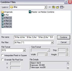 |
Combining files
is a two step process. The first step is to locate the images
you wish to combine using the combine tool under the
file menu. The more images the better, but in our case we
have 5 (only for are selected here, but all five images were
selected to create our bias frame.
|
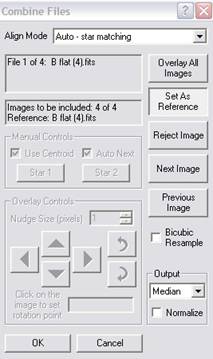 |
When the combine button is clicked, the second step of
the process is available. Auto – star matching is
selected automatically, but will be ignored in this case since
there are no stars to match. It is important to select median
under the output option. This averages the information in
all the images and combines them to a single master image. This
is the process that removed the white dot artifacts on the
individual bias images. This process of combining files to a
master file will work for both the bias and the flat images. Due
to the purpose of the star cluster images, the science images
are not to be combined! |
 |
The result of the
combine is an equally boring, but important image. In addition
to combing the bias frames, the flat frames will also be
combined. Since we are using BRI filters for our analysis, flat
frames for filters BRI are required; however, before any flat
frames are combined, the bias image must be applied to the flat
fields.
The
calibration tool, under the process menu has two
variants: set calibration or calibration wizard.
|
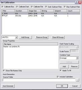 |
Version 4 of
MaxImDL has a very capable calibration wizard that I
highly suggest. The wizard walks you through the entire process.
The image on the left shows the calibration setting for the
science images, but the calibration tool can also use only the
bias image to calibrate the flat fields. Once the master bias
file is selected, simply open all of the flat frames and select
calibrate all under the process menu. This method
will also be used for the science images.
|
 |
 |
The image on the left
shows a single flat image (from the I flat field) and the image on the
right is a median combine of 5 flat images. This image will be used to
calibrate all of the science images using the I filter. The red and the
blue flat images look similar to the images above, and will not be
demonstrated to save space.
Using the same
calibration above, apply the calibration to the appropriate images.
Every image will use the master bias frame, but the filter specific
images will require the master file counterpart – i.e. images through
the B filter must be calibrated with the master bias and the master B
flat.
The result is a nicely
calibrated science image with no gross defects.
Now that we have
calibrated images, we can perform photometry on all the images. For the
purpose of calibration to the Landolt system, we will use images of
globular cluster NGC4147, Landolt Standard Area 104 (SA104), and Landolt
Standard Area 107 (SA107). As mentioned above, airmass plays a role in a
telescopes ability to ‘see’ a star. This affect can also interfere with
the color term. As a result, the fields NGC4147, SA104 and SA107 will be
images at various times through the night, so the position of these
areas will cause a difference in airmass value. These values, shown
later, will affect the outcome of the color term. The apparent magnitude
of selected stars in each of the calibration fields will need to be
documented. The best method is to use the photometry tool within
MaxImDL.
 |
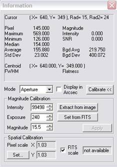 |
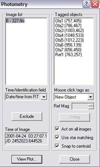
The photometry and
information windows work in tandem. In order to create a
photometry plot, a reference star is to be selected. A single reference
star from the Landolt standards can be selected, and the magnitude of
the reference star is required for the Ref Mag field. The
remaining stars are selected as objects. When the plot is viewed, the
results can be saved as a CSV (comma separated values) file.
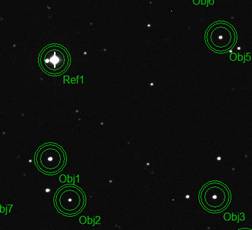 |
To the left is a
portion of an image being analyzed for photometry. The Ref1
is the reference star, and the Obj1, Obj2…... are the
object stars. Once the photometry plots are saved, the data can
be entered in an Excel spreadsheet. The attached spreadsheet
contains all of the instrument magnitudes of each filter (the
photometric data) as well as the Landolt standards.
|
Back to Top |
Back to
Astrophotography |