|
Color Magnitude Diagram of Cluster M67 - by Ricky Leon Murphy:
Introduction
Image Acquisition and Reduction
Calibration
The Color Magnitude Diagram
Analysis
Conclusion
References
Back to
Astrophotography
Introduction:
A color magnitude diagram is a
variant of the Hertzsprung-Russell diagram. While the Hertzsprung-Russell (H-R)
diagram is a summary of temperatures and magnitudes of individual stars, a color
magnitude diagram (CMD) is dedicated to the study of star clusters. The two most
common star clusters are globular and open. A globular cluster contains
thousands of stars and is considered old in comparison to other clusters (Ostlie,
page 529). They also tend to organize outside the main disk of a galaxy. Open
clusters on the other hand are considered young, and exist within the main disk
of a galaxy (Ostlie, page 530). The purpose of this project is to create a CMD
of an open cluster, M67, and give a brief analysis of the result. In order to
plot this diagram accurately, it is required that the images be calibrated to a
standard scale. Images are provided by Pamela Gay from the McDonald Observatory
in Davis Texas. In addition to images of M67, standard Landolt fields were
imaged, as well as the globular cluster NGC4147. The Landolt fields and NGC4147
will be used to create a calibration scale and the results applied to the images
of M67.
Back to Top
| Back to
Astrophotography
Image Acquisition and Reduction:
Use of spectral filters to
acquire an image is standard practice when imaging star fields for photometric
analysis; however, every telescope will influence the image with its color term.
In an effort to provide a standard, Arlo Landolt has created a system of
calibration based on the Johnson-Kron-Cousins photometric system. Using a
standard filter set, Professor Landolt cataloged 526 stars along the celestial
equator and documented each of these stars through UVBRI filters and averaged
the result (Landolt, 1992). These results are considered the standard
photometric system to which all other telescopes are to calibrate. The result of
this hard work is obvious: no mater the style, type, or size of a telescope, an
accurate CMD can be generated.
While the filters used for the
Landolt series were UVBRI, our diagram will be extrapolated from BRI images.
|
U filter |
Ultraviolet |
|
V filter |
Visible – or yellow |
|
B filter |
Blue |
|
R filter |
Red |
|
I filter |
Infrared |
The reason for selecting various
individual color filter images is to create a degree of magnitude difference
between them as an indication of color index – which can be translated to temperature.
Figure 1.
In addition to calibrating the
color term introduced by a telescope, the CCD camera used to acquire the images
must also be calibrated. While a single image from a CCD camera can be
calibrated to true black (using the overscan area), noise and heat induces small
changes in levels as more images are acquired. Because of this, an image called
a bias frame is required to calibrate every image according to the levels on
this one frame. In addition to the bias frame, a flat field must also be
captured. By capturing an image with the aperture blocked, noise and artifacts
are still acquired. When this image is applied to the other images, the majority
of noise and damage to the CCD chip will be subtracted from the image leaving
only the desired result. This entire process is called image reduction. MaxImDL
is used to calibrate the images, and extract photometric information from the
two given Landolt standard fields, NGC4147, and M67. Please see the appendix
Image Reduction – step by
step.
In addition to image reduction,
it is also necessary to create a photometric plot of each image. The process of
photometric extraction is also outlined in the Image Reduction – step by step
appendix. By selecting specific stars within the Landolt fields (fields SA104
and SA107 in this case) as well as specific stars indicated by Pamela Gay within
NGC4147, photometric information from the provided images are compared to the
Landolt standards.
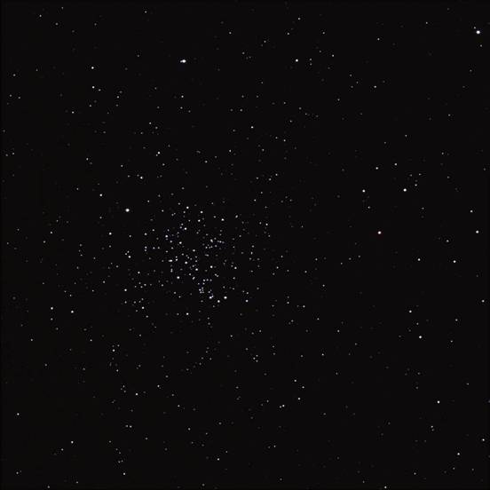
Our subject: M67 in RGB. The
green channel is synthetic, thanks to Registar.
Back to Top
| Back to
Astrophotography
Calibration:
The first step in calibration of
all the images is to organize the photometric data extracted by MaxImDL into an
Excel spreadsheet. The purpose of calibration is to determine the color term,
which is the value of a resulting mathematical expression used to compare
photometric results with a list of standard stars provided by the Landolt UVBRI
(BRI in our case) Photometric Standard Stars (Landolt, 1992). To solve for the
color term, the following equations are programmed into the attached Excel
spreadsheet, care of Pamela Gay:
mB = [(B-R) + R] + x1B
+ x2B ´ Airmass + x3B
´ (B-R),
mR = R + x1R
+ x2R ´ Airmass + x3R
´ (B-R),
mI = [R – (R – I)] +
x1I + x2I ´
Airmass + x3I ´ (R-I).
mB, mR, and mI
= instrument magnitude
B, R, I
= Landolt magnitude
x1
= constant
x2
= airmass
x3
= color term
In order to pinpoint the exact
color term of our telescope, we must plot scatter charts within Excel of the B,
R, and I images. Since Excel will be used to generate the scatter plots for
these three filters, it is easy to constrain the results to a standard deviation
of <0.2 and a median of 0 +/- 0.08 in comparison with the calculated Landolt
measurements – both are internal functions within the program.
Figure 2.
The plot above gives the slope of
instrument magnitudes compared to Landolt measured magnitudes for the B filter.
Figure 3.
The above plot is the slope of
the R filter images.
Figure 4.
This plot is the slope from the I
filter images.
|
Constants |
|
|
B |
R |
I |
|
x1 |
-0.3031 |
-0.2002 |
-0.3456 |
|
x2 |
-0.0338 |
0.0193 |
-0.0135 |
The resulting plots provides us
with the values for the constant (x1) and the color term of each filter (x2)
specific to the telescope used to
Figure 5.
capture the provided images.
The three plots above share the
same pattern: the horizontal axis is the calculated Landolt values: B-R for the
blue and red filters, and R-I for the infrared filter; the vertical axis is the
result of our instrument measurements with a constant and the airmass values in
comparison to the Landolt values. Specifically the plot for the blue and red
filters has the vertical values based on:
mB – B – b3 * XB and mR – R – r3 * XR,
where mB (mR) is the instrument
magnitude, B (R) is the Landolt magnitude, XB (XR) is the airmass value, b3 is a
constant value of 0.263 and r3 is a constant value of 0.159.
The term for the I filter is ignored since our CMD will plot stars based on the
B-R color index.
Back to Top
| Back to
Astrophotography
The Color Magnitude Diagram:
Now that all of the hard work is
out of the way, we can now concentrate on creating our very own CMD. With the
constants generated by the calibration method, we are now able to use the
photometry measurements of star cluster M67 and place it on a standard scale. To
make things simple, we will only create a CMD with a color index of B-R. The
magnitude of the stars representing the color index will run on the vertical
axis while the B-R will run on the horizontal axis.
The attached spreadsheet contains
the individual star data as well as the generated CMD. In order to put our plot
of M67 to the Landolt standards, two equations are used.
This first equation generates the
color term based on the selected stars:
B-R = (mB – mR) – (x1B – x1R) – (0.263 * XB – 0.159 * XR) / (1 + x2B – x2R)
Where x1B = -0.3031 (the constant
value from calibration), and x1R = -0.2002.
Once these values are calculated,
the standardized apparent magnitudes of the stars are calculated by:
R = (mR – x1R – x2R * BR – 0.159 * XR)
Where x2R = 0.0193 (the color
term), and BR is the value from the first equation.
For comparison purposes, let’s
take a look at a standard Hertzsprung-Russell (H-R) diagram:
Figure 6. (Image borrowed from:
http://www.astronomynotes.com/starprop/s13.htm)
Notice absolute magnitude scale
on the right and the B-V color on the bottom. Our CMD will have the same
orientation.
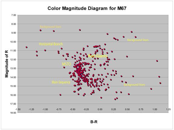
Figure 7.
With a sample of 373 stars, our
CMD contains enough information to make out several key features of this
diagram. At first glance, it would appear that the resulting graph is a
culmination of random stars; however, the concentration of stars near the center
has an appearance of a main-sequence belt. With the few background stars
ignored, it is also possible to see a group of stars populate the area
indicative of the red giant phase on the H-R diagram, as well as a possible
horizontal branch near the upper left of the diagram. Of significance is the
appearance of a clear cut-off of stars at the tip of the main-sequence. This
area refers to the main-sequence cut-off (MSTO) which is higher main-sequence
stars that have used up their supply of hydrogen, and are now in a core helium
burning stage. Since all the stars in a cluster form around the same time from
the same interstellar dust cloud, this cut-off demonstrates that the larger,
faster burning stars have already left the main-sequence and are populating the
red giant area of the diagram.
Back to Top
| Back to
Astrophotography
Analysis:
The study of a color magnitude
diagram can reveal a host of information about stellar evolution. With only 373
stars plotted on our diagram and only one color index featured, it would be
difficult to generate accurate information regarding stellar features such as
surface temperature, age, metallicity, and distance; however, we can infer with
reasonable certainty that our CMD can constrain these values to an acceptable
degree. With a B-R value of 1.03 (Doressoundiram, 2002), our Sun can serve as
the focal point so our CMD can be overlaid to a know H-R diagram (Figure 6).
Once the reference is made, we can clearly see that our CMD is composed of high
mass stars still residing on the main-sequence; while the higher mass stars have
successfully entered the red giant phase. It is safe to say that A and B
spectral type stars still exist on our main-sequence while the hottest O and OB
stars have turned off the main-sequence. With the A and B stars still on the
main-sequence, we can estimate this cluster is at least 15 x 10^6 years of age
(Freedman, page 481). With the bright B-R values of our plot, we can infer the
presence of abundant metals (Chiboucas, Internet) making the stars of our
cluster Population I stars. This is in agreement with open clusters being
younger in age that globular clusters. To estimate the distance to this cluster,
we will use the ever famous distance modulus:
m – M = 5 log d – 5.
Using our CMD as the guide, and
inserting the absolute magnitude of a star with a B-V
of 0, we know this B type star has an absolute magnitude of -2.
d = 10^(m-M+5)/5 pc.
d = 10^(15 – 2 + 5)/5 pc.
d = 3981 pc.
Back to Top
| Back to
Astrophotography
Conclusion:
By using a standard calibrating
system, we were able to calibrate images of star cluster M67. A color magnitude
diagram is a type of H-R diagram that is used as a tool in studying a star
cluster. Our CMD of M67 was able to reveal some very useful information. We are
able to determine that this cluster is metal rich, contains mostly high mass
stars, is around 15 x 10^6 years old, and has a distance of about 3900 parsecs.
While the information provided is only a rough estimate, it is clear that a CMD
has much to tell us. One of the most important aspects of a color magnitude
diagram is its ability to help us understand stellar evolution (Ostlie, page
531). It is also possible that CMD’s can provide valuable information to the
formation of white-dwarfs, and give insight to a fairly new stellar body called
the blue straggler.
We have much to learn about stellar evolution, but now we have the tools to help
us understand.
Back to Top
| Back to
Astrophotography
References:
Chiboucas, Kristin. “Research
Interests.”
http://www.astro.lsa.umich.edu/~kristin/html/interests.html
Doressoundiram, A. Et Al. “The
Color Distrobution in the Edgewoth-Kuiper Belt.” The Astrophysical Journal,
October 2002.
Freedman, Roger. William Kaufman.
Universe: Sixth Edition. W.H. Freeman and Company, New York. 2002.
Landolt, Arlo. “UBVRI Photometric
Standard Stars in the Magnitude Range 11.5 < V < 16.0 Around the Celestial
Equator.” The Astrophysical Journal, Volume 104, Number 1, July 1992.
Ostlie, Dale. Bradley Carroll.
An Introduction to: Modern Stellar Astrophysics. Addison-Wesley Publishing
Company, Massachusetts. 1996.
Hourly Airmass Table.
http://imagiware.com/astro/airmass.cgi. Internet.
Strobel, Nick. “Astronomy Notes.”
www.astronomynotes.com. Internet, 2004.
Back to Top |
Back to
Astrophotography |
